Given it’s a ring (i.e. not direction dependent), it’s very likely from something physically connected to the sonar. How have you mounted it to the bar? It’s possible the transmitted pulses are ringing through the chassis of the sonar, into the bar it’s mounted to, then bouncing back from the edges of the bar and appearing as a series of equally spaced rings.
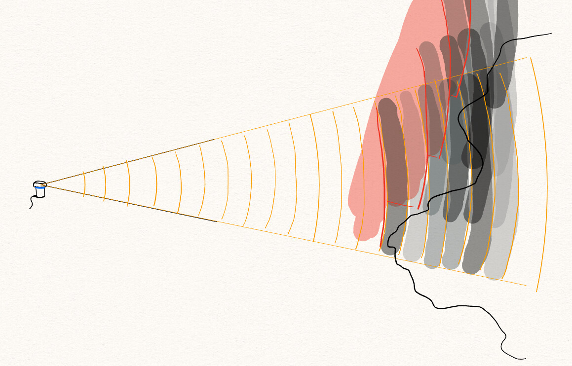
The core idea is to actually factor in the beam width and profile sample return strengths, then combine the regions of high response into the predicted surface, rather than just compressing each profile into a single distance estimate and creating a surface estimation from those points.
In the following profile, is the surface at the first strong response, or at the strongest response, or somewhere in between?
There isn’t necessarily a correct answer, and especially not one that generalises well to every individual profile.
The beam width is non-negligible (especially as compared to something like a laser, from a lidar scanner), and the spread can be simultaneously unhelpful for understanding where exactly the surface is, as well as very helpful for blocking out a large region where it isn’t.
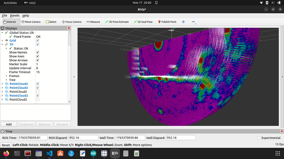
Consider the same scan with the sample return strengths, and in the context of some profiles that came before it:
The red regions had no response, so the surface isn’t there, and then the dip between the two peaks can potentially be detected using the regions where there are consistently strong returns between the different profiles. At the cost of some extra processing, the same scans can be combined to give a higher resolution, more accurate map of the surface.
In terms of actually implementing that, 3D Gaussians are seemingly a nice solution for modelling the spatial, density-like nature of the samples, particularly because:
- they can be stretched and arbitrarily oriented in space, which makes them well-suited to filling out slices of a beam,
- they have smooth boundaries, which matches the non-hard edges of the sonar beam, and allows easily adding up the effects of nearby gaussians without complex inclusion checks
- given they are functions of density, you could also specify negative densities for the regions where there was no response from a sample
- it is possible to fit a small set of Gaussians to approximate a larger set, which can avoid the need for explicit merging and/or culling when reducing a set of samples to a more manageable representation of the combined space
- they are defined about a central point, so region inclusion checks (e.g. when dealing with large numbers of Gaussians that have been limited to a maximum spread) can be performed efficiently using structures like octrees
- they can be rendered directly, using Gaussian splatting, which can (for some applications) avoid needing to generate a mesh to represent a surface (as would typically be required from a point cloud)